This guide shows how to perform quality control on a library using the barcoded constructs from the Minigene report and a sample sheet that contains a second, sample-level barcode.
The library itself is generated by ordering the barcoded constructs and then cloning them into the appropriate expression vectors to function as MHC-presented peptides. The sample barcode is then added via PCR primers and few rounds of amplification.
This workflow can be used either on the construct library, the transduced cells, or cells after co-culture. The goal of this step is to confirm that all constructs are present in the approriate proportions. We provide functions to process and analyze the sequencing data.
Preparation
Barcoded construct tables
The Minigene report step of this package provides a table with tiled reference and alternative peptides, along with their respective IDs. When ordering those as gene blocks, one or more construct barcodes are added to the sequence, so we are able to uniquely identify our minigene peptides also when a sequencing read does not reach the mutated base.
Here, we use barcodes from this publication and Github repository:
lib = "https://raw.githubusercontent.com/hawkjo/freebarcodes/master/barcodes/barcodes12-1.txt"
valid_barcodes = readr::read_tsv(lib, col_names=FALSE)$X1
These barcodes need to be of the same length and not overlap between samples in one QC run. For the analysis, we manually add them as columns to the peptide/minigene tables:
-
barcode– if only one barcode per construct -
barcode_1,barcode_2, etc. – if multiple barcodes per construct
The other required fields are, for each sample:
-
gene_name– an identifier for the gene, e.g.NRAS -
mut_id– a common identifier forrefandaltsequences, e.g.NRAS_Q61 -
pep_id– a unique identifier for each peptide, e.g.NRAS_Q61L-1 -
pep_type– whether this is areforaltsequence (or other) -
tiled– the tiled nucleotide sequence
For the QC analysis, we will need a named list of these barcoded
Minigene tables. We will usually have assembled them in a
.xlsx file with these barcodes added, however, here we will
use an example dataset:
## normally we'd read all sheets from our barcoded construct file:
# fname = "my_combined_barcoded_file.xlsx"
# sheets = readxl::excel_sheets(fname)
# all_constructs = sapply(sheets, readxl::read_xlsx, path=fname, simplify=FALSE)

all_constructs = example_peptides(valid_barcodes)We can confirm that these barcodes do not overlap:
plot_barcode_overlap(all_constructs, valid_barcodes)
#> Joining with `by = join_by(barcode)`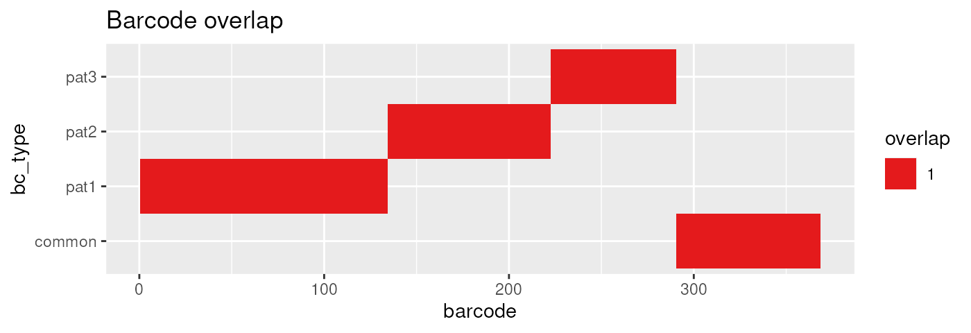
Creating a sample sheet
A sequencing (FASTQ) file will contain a sample barcode, construct barcode, and construct sequence:
fastq_file = "/path/to/your/file.fq.gz"Before we can start working with the FASTQ sequencing output, we need to describe which samples it contains. For this, we create a sample sheet with the following columns:
-
sample_id– a unique identifier of the sample -
patient– the patient or sample group that the sample comes from -
rep– a number indicating the replicate number -
origin– a descriptor of which kind of sample this is -
barcode– the barcode used to label all condition-specific constructs in the sequencing data
For this example, we have already provided a sample sheet with the
package. It includes three samples, two for library QC
(pat2 and pat3) and one with mock-transfected
vs. actual peptide T-cell co-culture (pat1). The
pat1 and pat2 samples additionally include a
common construct set. Whenever we use multiple construct sets in a
sample, we separate them using a +:
sample_sheet = system.file("my_samples.tsv", package="pepitope")Here, we did not actually do any sequencing, so we provide a simulated FASTQ file instead:
fastq_file = example_fastq(sample_sheet, all_constructs)Read structure and counting
Read structure definition
This step counts construct barcodes per sample directly from the
source FASTQ. Here, read_structure describes where the
sample and construct barcodes occur in each read. It has the following
possible fields, preceded by the number of nucleotides in the read. A
+ instead of a number is used to indicate to use all
remaining nucleotides:
-
B– the sample barcode to identify the sample (required) -
M– the construct barcode to count (required) -
T– the template read sequence (optional) -
S– skip these nucleotides and do not include in output (optional) -
^before a letter to denote a reverse complement sequence
In our example data, the sample barcode is followed directly by a reverse complement of the construct barcode, so the read structure is identified:
plot_read_structure(fastq_file, sample_sheet, all_constructs)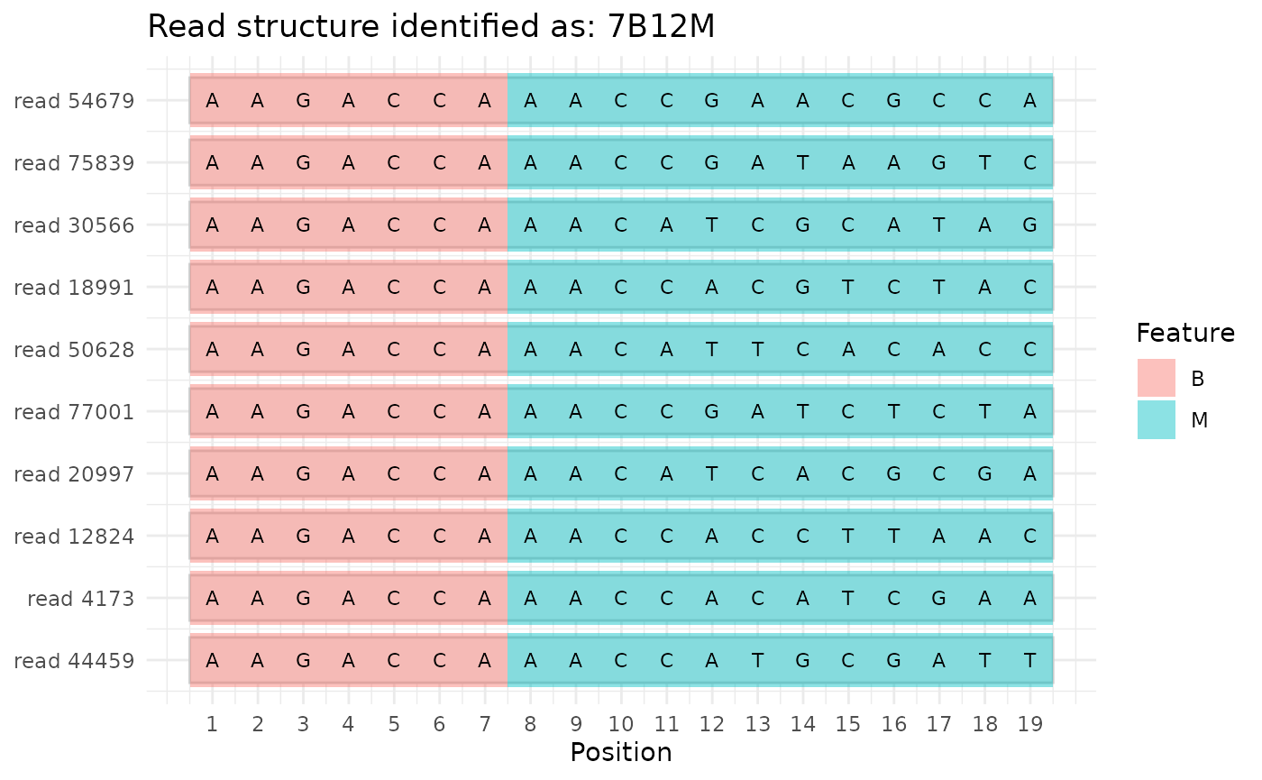
Counting sample and construct barcodes
In this example, the first 7 nucleotides identify the sample and the
next 12 nucleotides identify the construct are automatically inferred
from the read sequences. However, we could also specify it via the
read_structure argument:
dset = count_fastq(fastq_file, sample_sheet, all_constructs, valid_barcodes)
#> Read structure identified as '7B12M'
#> Counting barcodes in /tmp/RtmpBIVk2K/my_seqdata.fq
#> Processed 1,608,536 reads
Here, dset will be a SummarizedExperiment
object that you can interact with the following way:
-
colData(dset)– access the sample metadata asdata.frame -
rowData(dset)– access the construct metadata asdata.frame -
assay(dset)– access the construct counts asmatrix
Quality Control plots
Plotting total barcode counts
The first overview that we want to get is to know how many barcodes are in which demultiplexed FASTQ, and whether they match the sample we expect them to be from. We can plot this the following way, for total read counts on the top and number of barcodes that have 10 (default) or more reads on the bottom:
plot_read_count(dset, 10)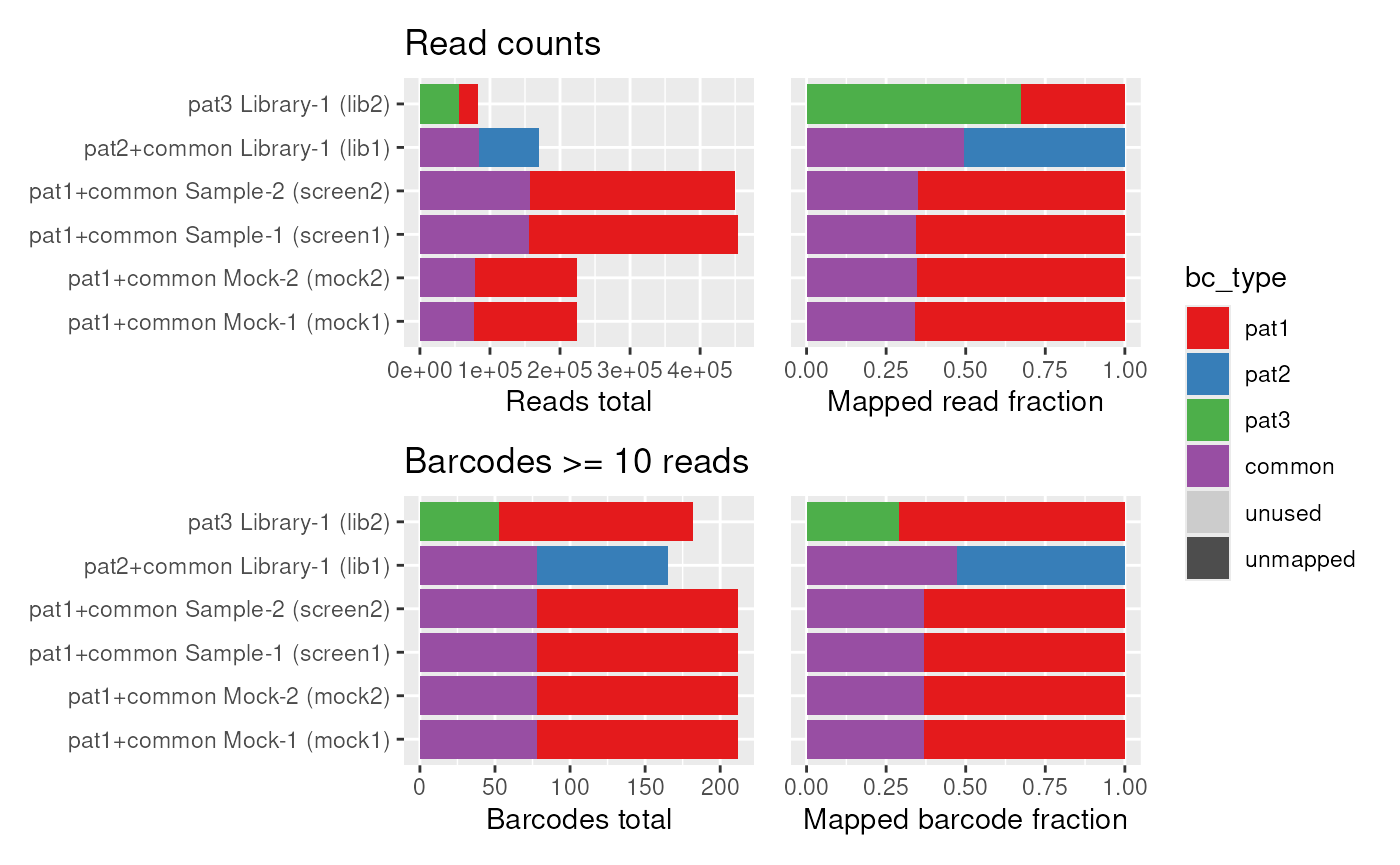
We can also plot this interactively with plotly:
Representation of individual barcodes
The next question we want to ask is whether the individual construct barcodes are equally distributed within a sample, and where any potential contaminations come from. For this, we order the barcodes from least abundant (left) to most abundant (right) and plot a continuous line for how many reads are sequenced of this barcode on the y axis:
plot_read_distr(dset)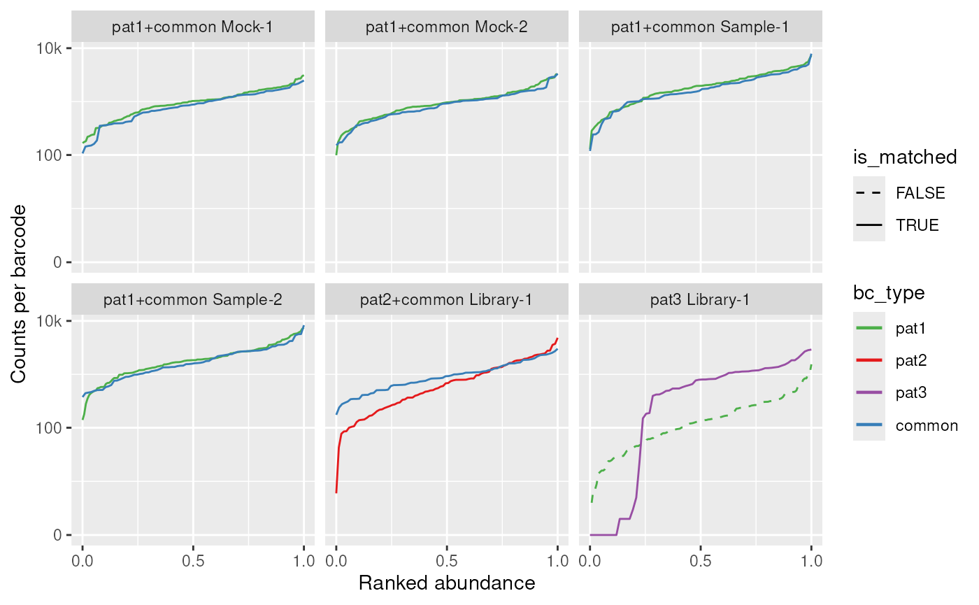
We can make a couple of observations from these plots:
- The
MockandSampleconditions worked well forpat1 - The sample-specific barcodes for
pat2show a high read variance and may be unsuitable for a screen - About a quarter of the sample-specific barcodes for
pat3are lost - There is a sample contamination of
pat1inpat3
We can also plot this interactively with plotly, where
we can hover over with the mouse to see which barcode is in which
position exactly:
library(plotly)
ggplotly(plot_read_distr(dset), height=500, tooltip="text")